Least Squares Theory
In the previous chapter, we talked about the Maximum Likelihood Estimator. However, MLE can be computationally difficult to calculate, often without analytical solutions, requiring iterative algorithms.
In this chapter, we introduce a series of “Least-Squares” estimators, that for a specific type of model (linear model), have fixed solutions derivable through minimisation. First, we introduce the classical linear model and its assumptions. Then, we discuss the most common least-square estimator: ordinary least squares (OLS). Finally, we discuss extensions to OLS (generalised least squares, instrumental variables) for when the assumptions needed for OLS are violated.
The Classical Linear Model
A class of estimators called least squares estimators is another way to estimate population parameters \(\theta\) besides MLE. However, this class of estimators can only be applied in one specific model: the classical linear model.
Let us say there are individuals \(t = 1, 2, \dots, n\) in the population. Each individual’s \(Y\) value is determined by a set of random variables \(Y_1, \dots, Y_n\). Any individual random variable \(Y_t\) is data generating process defined as \(Y_t \sim \set D(\mu_Y, \sigma^2_Y)\), where \(\set D\) represents any distributional form, \(\mu_Y\) is the mean of the random variable, and \(\sigma^2_Y\) is the variance of the random variable.
The classical linear model is a specification that the mean \(\mu_Y\) of \(Y_t\) is linearly determined by a set of explanatory variables \(\set X = \{X_1, \dots, X_p\}\):
\[ \E(Y_t|\set X_t) = \beta_0 + \beta_1 X_{1t} + \beta_2 X_{2t} + \dots + \beta_p X_{pt} \]
Where \(\beta_0, \dots, \beta_p\) are a set of population parameters (that need to be estimated) that determine how \(\mu_Y\) changes in respect to explanatory variables \(\set X\).
You will frequently see the linear model represented in another form:
\[ Y_t = \underbrace{\beta_0 + \beta_1 X_{1t} + \dots + \beta_p X_{pt}}_{\E(Y_t | \set X_t)} + \eps_t, \quad \eps_t \sim \set D(\mu_{\eps_t} = 0, \sigma^2_{\eps_t}) \]
Where the error term \(\eps_t\) represents the variance/randomness in our data generating process, and the rest of the model represents \(\mu_y\).
We know that this data generating process applies for random variables \(Y_1, Y_2, \dots, Y_n\). To represent all random variables together, we use the matrix representation of the linear model:
\[ \b y = \b{X\beta} + \b\eps \iff \begin{pmatrix} y_1 \\ y_2 \\ \vdots \\ y_n\end{pmatrix} = \begin{pmatrix} 1 & x_{11} & \dots & x_{1p} \\ 1 & x_{21} & \dots & x_{2p} \\ \vdots & \vdots & \dots & \vdots \\ 1 & x_{n1} & \dots & x_{np}\end{pmatrix} \begin{pmatrix} \beta_0 \\ \beta_1 \\ \vdots \\ \beta_p\end{pmatrix} + \begin{pmatrix} \eps_1 \\ \eps_2 \\ \vdots \\ \eps_n \end{pmatrix} \]
The classical linear model has a set of five assumptions:
Definition 4.1 (Linearity in Parameters) A model is linear in parameters if it can be written in the form \(\b y = \b{X\beta} + \b \eps\). Or in other words, all parameters \(\beta_0, \dots, \beta_p\) must be either added or subtracted from each other.
It is important to note that linearity in parameters is not equal to linearity in the classical sense. For example, the model
\[ Y_t = \beta_0 + \beta_1X_t + \beta_2 X_t^2 + \beta_3X_t^3 + \eps_t \]
would be considered linear in parameters because all parameters \(\beta_0, \dots, \beta_p\) are added together, not multiplied. It does not matter if the \(X\) are linear or not.
Definition 4.2 (Independent and Identically Distributed) A series of random variables \(Y_1, Y_2, \dots, Y_n\) is considered to be independent and identically distributed if each random variable is independent (definition 1.6), and each random variable has the exact same distribution.
This assumption is often not met in its purest form - since when we randomly sample \(Y_t\) without replacement, technically the next observation \(Y_{t+1}\) will have slightly different distribution, since we took one observation out already.
This assumption is also frequently violated in time-series data, where \(Y_t\) at time \(t\) is likely to have an effect on \(Y_{t+1}\) at time \(t+1\).
Definition 4.3 (Linear Independence) Also called non-perfect multicollinearity, this assumption means that no explanatory variables \(X_1, \dots, X_p\) can be perfectly correlated with any other explanatory variable, or perfectly correlated with any linear combination of other explanatory variables.
This assumption is required for estimation to be possible with the ordinary least squares estimator, as it requires matrix \(\b X\) to be full rank which allows \(\b X^\top \b X\) to be invertable.
Definition 4.4 (Strict Exogeneity) Strict Exogeneity is \(\E(\b\eps | \b X) = 0\). This implies that \(\E(\b X^\top \b\eps) = 0\), which means all regressors \(X_1, \dots, X_p\) should be uncorrelated with the error terms \(\eps\), and any linear combination of \(X_1, \dots, X_p\) should be uncorrelated with the error term.
There is also a weaker form of exogeneity, called weak exogeneity:
Definition 4.5 (Weak Exogeneity) Weak exogeneity is defined as \(\E(\b x_t \eps_t) = 0\). Weak exogeneity only requires that regressors \(X_1, \dots, X_p\) individually are uncorrelated with the error term. Weak exogeneity allows for combinations of \(X_1, \dots, X_p\) to to be correlated with \(\eps\), which is not allowed under strict exogeneity.
Definition 4.6 (Spherical Errors) The spherical errors assumption states that the covariance matrix of errors \(\eps_t\) takes the form:
\[ \V(\b\eps|\b X) = \sigma^2 \b I_n = \begin{pmatrix} \sigma^2 & 0 & 0 & \dots \\ 0 & \sigma^2 & 0 & \dots \\ 0 & 0& \sigma^2 & \vdots \\ \vdots & \vdots & \dots & \ddots \end{pmatrix} \]
The variance-covariance matrix of errors \(\eps_t\) takes the form:
\[ \V(\b\eps | \b X) = \b\Omega = \begin{pmatrix} \V \eps_1 & Cov(\eps_1, \eps_2) & Cov(\eps_1, \eps_3) & \dots \\ Cov(\eps_2, \eps_1) & \V \eps_2 & Cov(\eps_2, \eps_3) & \dots \\ Cov(\eps_3, \eps_1) & Cov(\eps_3, \eps_2) & \V\eps_3 & \vdots \\ \vdots & \vdots & \dots & \ddots \end{pmatrix} \]
Spherical errors implies two things:
- No Autocorrelation means that the covariance of any two error terms \(Cov(\eps_i, \eps_j) = 0\). This is reflected in spherical errors with all the 0’s in the non-diagonal positions.
- Homoscedasticity means that every \(\eps_t\) for any observation \(t\) has the same variance \(\sigma^2\). The variance of the error \(\eps_t\) does not depend on the values of \(X_1, \dots, X_p\). If this condition is violated, as in each observation \(t\) has their own \(\sigma^2_t\), we call this homoscedasticity.
Ordinary Least Squares
OLS is an estimation process that finds the values \(\hat{\b\beta}\) by the \(\hat{\b\beta}\) values that minimise the sum of squared residuals (SSR) (also called the sum of squared errors), the difference between \(\b y\) and predicted \(\hat{\b y}\) squared, where \(\hat{\b y}\) is defined as \(\hat{\b y} = \b X \hat{\b\beta}\).
Definition 4.7 (Sum of Squared Residuals) We will define the SSR by function \(S(\hat{\b\beta})\):
\[ S(\hat{\b\beta}) = \sum\limits_{i=1}^n (Y_i - \hat Y_i)^2 \ = \ (\b y - \hat{\b y})^\top (\b y - \hat{\b y}) \]
One common question is why are we squaring the residuals (difference between \(\b y\) and \(\hat{\b y}\)). The main reason is that squaring gets rid of negative and positive residuals, which might cancel each other out. We do not care about the direction of residuals/errors, only the magnitude.
The reason we choose to square the residuals, and not to use absolute value, is because of a variety of unique properties of OLS (unbiasedness, variance, efficeincy) that we will explore throughout this chapter.
We know that predicted \(\hat{\b y} = \b X \hat{\b \beta}\). Thus, let us plug that into \(S(\hat{\b\beta})\), and simplify to get:
\[ \begin{align} S(\hat{\b\beta}) & = (\b y - \b X \hat{\b\beta})^\top (\b y - \b X \hat{\b\beta}) \\ & = \b y^\top \b y - \hat{\b\beta}^\top \b X^\top \b y - \b y^\top \b X \hat{\b\beta} + \hat{\b\beta}^\top \b{X^\top X} \hat{\b\beta} \\ & = \b y^\top \b y - 2 \hat{\b\beta}^\top \b{X^\top y} + \hat{\b\beta}^\top \b{X^\top X} \hat{\b\beta} \end{align} \]
Now, we want to maximise in respect to \(\hat{\b\beta}\), so let us take the gradient of function \(S\) in respect to \(\hat{\b\beta}\), and set it equal to 0. Then, we can solve for \(\hat{\b\beta}\) to get our parameter estimates:
\[ \begin{align} \frac{\partial S}{\partial \hat{\b\beta}} = -2 \b{X^\top y} + 2 & \b{X^\top X} \hat{\b\beta} = 0 \\ 2 \b{X^\top X}\hat{\b\beta} & = 2 \b{X^\top y} \\ \hat{\b\beta} & = (2 \b{X^\top X})^{-1}2 \b{X^\top y} \\ \hat{\b\beta} & = (2^{-1})2(\b{X^\top X})^{-1}\b{X^\top y} \\ \hat{\b\beta} & = (\b{X^\top X})^{-1}\b{X^\top y} \end{align} \]
Definition 4.8 (OLS Estimate) The OLS estimate of parameters \(\b\beta\) is:
\[ \hat{\b\beta}_{\mathrm{OLS}} = (\b{X^\top X})^{-1}\b{X^\top y} \]
For simple linear regression, our sum of squared errors (definition 4.7) is:
\[ S(\hat\beta_0, \hat\beta_1) = \sum\limits_{t=1}^n (Y_t - \hat\beta_0 - \hat\beta_1 X_t)^2 \]
Our first order conditions by taking the partial derivative in respect to \(\hat\beta_0\) and \(\hat\beta_1\) are:
\[ \begin{align} & \frac{\partial S}{\partial \hat\beta_0} = \sum\limits_{i=1}^n (Y_t -\hat\beta_0 = \hat\beta X_t) = 0 \\ & \frac{\partial S}{\partial \hat\beta_1} = \sum\limits_{i=1}^n X_t (Y_t -\hat\beta_0 = \hat\beta X_t) = 0 \\ \end{align} \]
And the final solutions for \(\hat\beta_0\) and \(\hat\beta_1\) after solving this system of equations is:
\[ \begin{align} & \hat\beta_0 = \bar Y - \hat\beta_1 \bar X \\ & \hat\beta_1 = \frac{\sum (X_t -\bar X)(Y_t -\bar Y)}{\sum (X_t - \bar X)^2} = \frac{Cov(X, Y)}{\V Y} \end{align} \]
OLS has some unique properties, that we will explore in the tabs below.
Recall our predictions \(\hat{\b y} = \b X \hat{\b\beta}\). Using our OLS solution, we can find
\[ \hat{\b y} = \b X (\b{X^\top X})^{-1} \b{X^\top y} = \color{red}{\b P}\color{black}{\b y} \]
Definition 4.9 (Projection Matrix) Let us define the projection matrix \(\b P\) as:
\[ \color{red}{\b P}\color{black} := \b X(\b{X^\top X})^{-1} \b X^\top \]
Matrix \(\color{red}{\b P}\) is symmetrical as in \(\b P^\top = \b P\), and is idempotent as in \(\b{PP} = \b P\).
We can see that projection matrix \(\color{red}{\b P}\) performs a linear mapping of \(\b y \rightarrow \hat{\b y}\), hence why it is called the “projection” matrix.
Now, let us look at our residuals \(\hat{\b \eps} = \b y - \hat{\b y}\). By plogging in \(\b y = \b{Py}\), we can get:
\[ \hat{\b\eps} = \b y - \color{red}{\b P} \color{black}{\b y} = (\b I - \color{red}{\b P}\color{black})\b y = \color{purple}{\b M} \color{black}{\b y} \tag{4.1}\]
Definition 4.10 (Residual Maker Matrix) Let us define the residual maker matrix \(\b M\) as:
\[ \color{purple}{\b M}\color{black} := \b I - \b X(\b{X^\top X})^{-1} \b X^\top = \b I - \color{red}{\b P} \]
Matrix \(\color{purple}{\b M}\) is symmetrical as in \(\b M^\top = \b M\), and is idempotent as in \(\b{MM} = \b M\). Residual maker \(\b M\) is also orthogonal to \(\b P\) and \(\b X\), implying \(\b{PX} = 0\) and \(\b{MX} = 0\).
We can see that residual maker matrix \(\color{purple}{\b M}\) performs a linear mapping of \(\b y \rightarrow \hat{\b\eps}\), thus “making” the residuals \(\hat{\b\eps}\).
From the previous tab, we see projection matrix \(\color{red}{\b P}\) performs a linear mapping of \(\b y \rightarrow \hat{\b y}\), hence why it is called the “projection” matrix. We can see that residual maker matrix \(\color{purple}{\b M}\) performs a linear mapping of \(\b y \rightarrow \hat{\b\eps}\), thus “making” the residuals \(\hat{\b\eps}\).
We know that our predictsion \(\hat{\b y}\) are a linear combination of our explanatory variable vectors \(X_1, \dots, X_p\), since \(\hat{\b y} = \b X \hat{\b\beta}\). This means that projection matrix \(\color{red}{\b P}\) projects \(\b y\) into \(\hat{\b y}\) which is in the space spanned by our \(\b X\) (called the column space of \(\b X\)).
This is visualised in the figure below, where observed vector \(\b y\) is projected into the blue space of regressors \(\b X\) to create vector \(\hat{\b y}\):
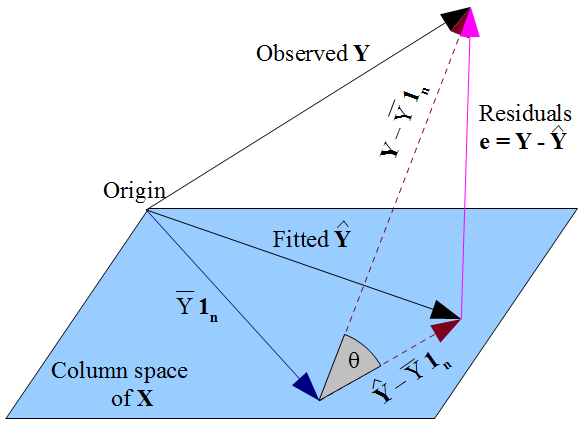
We can see as well that residual maker \(\color{purple}{\b M}\) projects vector \(\b y\) into vector \(\b\eps\), which is in the space orthogonal/perpendicular to the column space of \(\b X\). This is why our condition of strict exogeneity (definition 4.4) is required - there should be no correlation between \(\b X\) and \(\b \eps\) as they are orthogonal by design.
This idea of projection from the last tabe means we can measure the fit of our model with the correlation/overlap between original vector \(\b y\) and our predicted values vector \(\hat{\b y} = \b{Py}\).
Definition 4.11 (R-Squared) \(R^2\) is a metric to measure the fit of our model.
\[ R^2 = \frac{\overbrace{\b{y^\top Py}}^{\text{model}}}{\underbrace{\b{y^\top y}}_{\V Y}} \ = \ 1-\frac{\overbrace{\sum(Y_t - \hat Y_t)^2}^{\text{SSR}}}{\underbrace{\sum (Y_t - \bar Y)^2}_{\V Y}} \]
\(R^2\) is always between 0 and 1, and measures the proportion of variance our model with explanatory variables \(X_1, \dots, X_p\) explains the variation in \(Y\).
The first definition of \(R^2\) works because a dot-product of vectors measures their overlap/shadow on each other - so \(\b{y^\top Py}\) measures the overlap between our actual \(\b y\) and our model \(\b{Py}\). This is divided by the maximum possible shadow of \(\b y\) on itself, to ensure a \(R^2\) between 0 and 1.
The second definition of \(R^2\) works because we know the SSR is the part of \(Y\) that is not explained by our model (the error). Thus, SSR divided by the variance in \(Y\) is the porportion of the variance in \(Y\) not explained by our model. Thus, the remaining part must be explained by our model, so we do 1 minus SSR/Variance.
A partitioned regression model is when we split up our matrices/vectors in our classical linear model \(\b y = \b{X\beta} + \b\eps\). Let us say we only care about some of the explanatory variables in our data generating process. We can split matrix \(\b X\) into two: \(\b X_1\) contains the explanatory variables we care about, and \(\b X_2\) contains the other explanatory variables. Similarly, we divide \(\b\beta\). We get:
\[ \b y = \b X_1 \b\beta_1 + \b X_2 \b\beta_2 + \b\eps \]
Recall the residual maker matrix \(\b M\) (definition 4.10), and recall how \(\b M\) is orthogonal to \(\b X\), meaning \(\b{MX} = 0\). Now, let us consider only the residual maker matrix of the second part of our partitioned model \(\b M_2\), which means \(\b M_2 \b X_2 = 0\). Let us take our partitioned regression model, and pre-multiply \(\b M_2\) to both sides:
\[ \begin{align} \b M_2 \b y & = \b M_2(\b X_1 \b\beta_1 + \b X_2 \b\beta_2 + \b\eps) \\ \b M_2 \b y & = \b M_2 \b X_1 \b\beta_1 + \b M_2 \b X_2 \b\beta_2 + \b M_2 \b\eps \end{align} \]
Now recall that \(\b M_2 \b X_2 = 0\). That means we can simplify the above to
\[ \b M_2 \b y = \b M_2 \b X_1 \b\beta_1 + \b M_2 \b\eps \]
Now, let us define \(\tilde{\b y} := \b M_2 \b y\), \(\tilde{\b X_1} := \b M_2 \b X_1\), and error \(\tilde{\b\eps} = \b M_2 \b\eps\). We can rewrite as
\[ \tilde{\b y} = \tilde{\b X_1}\b\beta_1 + \tilde{\b \eps} \]
Using definition 4.8, we know the OLS estimate of \(\hat{\b \beta_1}\) is:
\[ \hat{\b\beta}_1 = (\tilde{\b X_1^\top} \tilde{\b X_1}) \tilde{\b X_1^\top} \tilde{\b y} \]
\(\hat{\b\beta}_1\) is equal to our normal OLS estimates without partitioning the model. Notice how we have \(\tilde{\b X_1} := \b M_2 \b X_1\) in our formula. Well, we know \(\b M_2 \b X_2 = 0\). That means that any part of \(\b X_1\) that was correlated to \(\b X_2\) became 0, after it was multiplied by \(\b M_2\). Thus, \(\tilde{\b X_1}\) is the part of \(\b X_1\) that is uncorrelated with \(\b X_2\).
Theorem 4.1 (Regression Anatomy Theorem) Our individual parameter estimates \(\hat\beta_j \in \{\hat\beta_1, \dots, \hat\beta_p \}\) are the relationship between \(Y\) and the part of \(X_j \in \{X_1, \dots, X_p\}\) uncorrelated with the other explanatory variables.
OLS Estimator Properties
We know that an estimator has two finite sample properties: unbiasedness (definition 2.4) and variance (definition 2.5), and has the asymptotic property of consistency (definition 2.6). Before we explore these properties, let us first transform our OLS estimates (definition 4.8) into a form more useful for showing these properties of OLS.
Let us start with our OLS solution (definition 4.8), and plug in our original model \(\b y = \b{X\beta} + \b\eps\) into where \(\b y\) is in the OLS solution:
\[ \begin{align} \hat{\b\beta} & = (\b{X^\top X})^{-1} \b{X^\top y} \\ & = (\b{X^\top X})^{-1} \b X^\top (\b{X\beta} + \b\eps) \\ & = \underbrace{(\b{X^\top X})^{-1}\b{X^\top X}}_{\text{inverses cancel}}\b\beta + (\b{X^\top X})^{-1} \b{X^\top \eps} \\ & = \b\beta + (\b{X^\top X})^{-1}\b{X^\top \eps} \end{align} \tag{4.2}\]
Now, we are ready to explore the properties of the ordinary least squares estimator: unbiasedness, variance, and consistency.
Theorem 4.2 (OLS is an Unbiased Estimator) The Ordinary Least Squares estimator is an unbiased estimator under the assumptions of linearity, i.i.d., linear independence, and strict exogeneity.
\[ \E \hat{\b\beta} = \b\beta \]
Note that the assumption of spherical errors is not needed for the unbiasedness of OLS.
Proof: Let us take the expectation of \(\hat{\b\beta}\) (from eq. 4.2) conditional on \(\b X\) (remember that \(\b X\) and \(\b \beta\) are fixed constants, so they are not affected by the expectation). We can use the strict exogeneity assumption (definition 4.4) to simplify:
\[ \E(\hat{\b\beta}|\b X) = \b\beta + (\b{X^\top X})^{-1} \underbrace{\E (\b \eps | \b X)}_{= \ 0} = \b\beta \]
Now, we know \(\E(\hat{\b\beta} | \b X)\). We can deduce \(\E(\hat{\b\beta})\) using the law of iterated expectations (theorem 1.3), and plugging in \(\E(\hat{\b\beta} | \b X) = \b\beta\):
\[ \E(\hat{\b\beta}) = \E[\E(\hat{\b\beta}|\b X)] = \E[\b\beta] = \b\beta \]
The final step is because the expectation of a constant \(\b\beta\) (the fixed true population value) is the constant itself. Thus, we have proven OLS is an unbiased.
Theorem 4.3 (Variance of the OLS Estimator) The variance of the OLS estimator under the assumptions of linearity, i.i.d., linear independence, strict exogeneity, and spherical errors, is given by
\[ \V(\hat{\b\beta}|\b X) = \sigma^2 (\b{X^\top X})^{-1} \]
Proof: Let us start where we left off from eq. 4.2. This tells us the variance of the OLS estimator is:
\[ \V(\hat{\b\beta}|\b X) = \V(\b\beta + (\b{X^\top X})^{-1} \b{X^\top \eps}) \]
We know that \(\b\beta\) is a vector of fixed true population values. \((\b{X^\top X})^{-1} \b X^\top\) can also be considered a fixed constant matrix because we are conditioning our variance on \(\b X\). Thus, we can use theorem 1.2 to rewrite the above as
\[ \V(\hat{\b\beta}|\b X) = (\b{X^\top X})^{-1}\b X^\top \V(\b\eps| \b X)[(\b{X^\top X})^{-1}\b X^\top]^{-1} \]
With the properties of matrix inverses and transposes, we can determine that \([(\b{X^\top X})^{-1}\b X^\top]^{-1}\) is equivalent to \(\b X(\b{X^\top X})^{-1}\). Thus, plugging this in, we get
\[ \V(\hat{\b\beta}|\b X) = (\b{X^\top X})^{-1}\b X^\top \V(\b\eps| \b X) \b X(\b{X^\top X})^{-1} \]
Now, according to the assumption of spherical errors (definition 4.6), we know that \(\V(\b \eps| \b X) = \sigma^2 \b I_n\). Thus, let us plug that into our equation to get
\[ \V(\hat{\b\beta}|\b X) = (\b{X^\top X})^{-1}\b X^\top \sigma^2 \b I_n \b X(\b{X^\top X})^{-1} \]
Since \(\b I_n\) is the identity matrix, it cancels out. For notation simplicity, we can move the scalar \(\sigma^2\) to the front, and simplify:
\[ \begin{align} \V(\hat{\b\beta}|\b X) & = \sigma^2 \underbrace{(\b{X^\top X})^{-1}\b X^\top \b X}_{\text{inverses cancel}}(\b{X^\top X})^{-1} \\ & = \sigma^2 (\b{X^\top X})^{-1} \end{align} \]
Thus, we have proved that the variance of the OLS estimator is as the theorem above.
Theorem 4.4 (Consistency of OLS) The Ordinary Least Squares estimator is asymptotically consistent (definition 2.6), under the assumptions of linearity, i.i.d., linear independence, weak exogeneity, and spherical errors. Mathematically:
\[ \mathrm{plim}\hat{\b\beta} = \b\beta \]
Proof: Let us start off from eq. 4.2. We can rewrite our matrix notation in the form of vectors, scalars, and summation:
\[ \begin{align} \hat{\b\beta} & = \b\beta + (\b{X^\top X})^{-1}\b{X^\top\eps} \\ & = \b\beta + \left(\sum\limits_{t=1}^n \b x_t \b x_t^\top\right)^{-1} \left(\sum\limits_{t=1}^n\b x_t \eps_t \right) \end{align} \]
Now, let us do a little algebra trick as follows:
\[ \hat{\b\beta} = \b\beta + \left(\frac{1}{n}\sum\limits_{t=1}^n \b x_t \b x_t^\top\right)^{-1} \left(\frac{1}{n}\sum\limits_{t=1}^n\b x_t \eps_t \right) \]
The reason we can do this is because the first \(\frac{1}{n}\) is inversed as \(\frac{1}{n}^{-1}\), so this cancels out the second one, maintaining the equality of our equation.
Now, we want to prove \(\mathrm{plim}\hat{\b\beta} =\b\beta\), so let us take the probability limit of both sides.
\[ \mathrm{plim}\hat{\b\beta} = \mathrm{plim} \b\beta + \left( \mathrm{plim} \frac{1}{n}\sum\limits_{t=1}^n \b x_t \b x_t^\top \right)^{-1} \left( \mathrm{plim}\frac{1}{n}\sum\limits_{t=1}^n\b x_t \eps_t \right) \]
We know that the probability limit of a constant is itself, so \(\mathrm{plim} \b\beta = \b\beta\), since \(\b\beta\) is a constant of true population parameters. Look at the other two terms on the right. They take the form of sample averages \(\frac{1}{n}\sum\). Using the law of of large numbers (theorem 2.1), we can simplify to:
\[ \mathrm{plim}\hat{\b\beta} = \b\beta + (\E(\b x_t \b x_t^\top))^{-1} \underbrace{\E(\b x_t \eps_t)}_{=0} = \b\beta \]
And we know \(\E(\b x_t \eps_t) = 0\) because of the condition of weak exogeneity (definition 4.5). Thus, we have proved that OLS is asymptotically consistent.
Gauss-Markov Theorem
You might ask, what is so special about Ordinary Least Squares, and why should we use this estimator? The answer lies in the Gauss-Markov Theorem.
Theorem 4.5 (Gauss-Markov) If all of the assumptions of linearity, i.i.d., no perfect multicollinearity, strict exogeneity, and spherical errors are all met, then the Ordinary Least Squares estimator is the best linear unbiased estimator (BLUE) - the unbiased linear estimator with the lowest variance of any other unbiased estimator.
Formally, if \(\hat{\b\beta}\) is the OLS estimator, and \(\tilde{\b\beta}\) is any other linear unbiased estimator, then
\[ \V(\hat{\b\beta}|\b X) ≤ \V(\tilde{\b\beta} | \b X) \]
Any linear estimator \(\tilde{\b\beta}\) must be in the form \(\tilde{\b\beta} = \b{Cy}\), where \(\b C\) is some linear mapping. For example, using projection matrix \(\b P\) (definition 4.9), OLS can be written as \(\hat{\b\beta} = \b{Py}\). Before we prove the Gauss-Markov theorem, we need a lemma about any unbiased linear estimator.
Lemma 4.1 For any linear estimator \(\tilde{\b\beta} = \b{Cy}\) to be unbiased, \(\b{CX} = \b I\).
Proof: Let us start off with our linear estimator \(\tilde{\b\beta} = \b{Cy}\), and plug in the true linear model \(\b y = \b{X\beta} + \b\eps\) into our linear estimator:
\[ \tilde{\b\beta} = \b C (\b{X\beta} + \b\eps) = \b{CX\beta} + \b{C\eps} \]
Now, let us find the expected value of this estimator conditional on \(\b X\). Remember that the expected values of constants (like \(\b C\), \(\b \beta\), and \(\b X\) since we are conditioning on \(\b X\)) are the constants themselves.
\[ \begin{align} \E(\tilde{\b\beta}|\b X) & = \E(\b{CX\beta} + \b{C\eps}) \\ & = \b{CX\beta} + \b C \E(\b\eps| \b X) \end{align} \]
From the strict exogeneity assumption (definition 4.4), we know \(\E(\b\eps | \b X) = 0\), so we can simplify to
\[ \E(\tilde{\b\beta}|\b X) = \b{CX\beta} \]
And using the law of iterated expectations (theorem 1.3), we can find \(\E\tilde{\b\beta}\):
\[ \E\tilde{\b\beta} = \E[\E(\tilde{\b\beta}|\b X)] = \E[\b{CX\beta}] = \b{CX\beta} \]
For unbiasedness (definition 2.4), we know \(\E\tilde{\b\beta} = \b\beta\). The only way \(\b{CX\beta}\) will equal \(\b\beta\) is if \(\b{CX} = \b I\). Thus, for any linear unbiased estimator, the lemma \(\b{CX} = \b I\) must hold.
With this lemma, now let us prove Gauss-Markov. First, let us calculate the variance of unbiased linear estimator \(\tilde{\b\beta}\):
\[ \begin{align} \V(\tilde{\b\beta} | \b X) & = \V(\b{Cy} | \b X) \\ & = \V(\b C( \b{X\beta} + \b \eps)| \b X) \\ & = \V(\b{CX\beta} + \b{C\eps} | \b X) \end{align} \]
And since we know from Lemma 4.1 that \(\b{CX = I}\), we can get
\[ \V(\tilde{\b\beta} | \b X) = \V(\b\beta + \b{C\eps} | \b X) \]
We know that \(\b\beta\) is a vector of fixed constants (the true population values). We also know \(\b C\) is some fixed constant matrix (that depends on \(\b X\), but we are conditioning on \(\b X\)). Thus, we can use theorem 1.2 to rewrite the above as
\[ \V(\tilde{\b\beta} | \b X) = \b C\V(\b\eps | \b X) \b C^\top \]
Now, according to the assumption of spherical errors (definition 4.6), we know that \(\V(\b \eps| \b X) = \sigma^2 \b I_n\). Thus, let us plug that into our equation to get
\[ \begin{align} \V(\tilde{\b\beta} | \b X) & = \b C \sigma^2 \b I_n \b C^\top \\ & = \sigma^2 \b{CC^\top} \end{align} \tag{4.3}\]
Now we have the variance of estimator \(\tilde{\b\beta}\). To prove Gauss-Markov, we need to show that the variance of \(\tilde{\b\beta}\) is greater than the variance of \(\hat{\b\beta}\). For this to be true,
\[ \V(\tilde{\b\beta}|\b X) - \V(\tilde{\b\beta}| \b X) ≥ 0 \]
We can plug in the variance of \(\tilde{\b\beta}\) from eq. 4.3, and the variance of OLS \(\hat{\b\beta}\) from theorem 4.3:
\[ \begin{align} \sigma^2 \b{CC^\top} - \sigma^2 (\b{X^\top X})^{-1} & ≥ 0 \\ \sigma^2 (\b{CC^\top} - (\b{X^\top X})^{-1}) & ≥ 0 \end{align} \]
We know from Lemma 4.1 that \(\b{CX} = \b I\), which through the properties of tranposes, also implies that \(\b{X^\top C^\top} = (\b{CX})^\top = \b I\). Multipling by \(\b I\) doesn’t change anything, so we can insert a \(\b{CX}\) and \(\b{X^\top C^\top}\) into our equation above to get
\[ \sigma^2 (\b{CC^\top} - \b{CX} (\b{X^\top X})^{-1}\b{X^\top C^\top}) ≥ 0 \]
Factoring out \(\b C\) and \(\b C^\top\), and remembering our residual maker \(\b M\) (definition 4.10),
\[ \begin{align} \sigma^2 \b C(\b I - \b X(\b{X^\top X}^{-1}\b X^\top) \b C^\top & ≥ 0 \\ \sigma^2 \b{CMC} & ≥ 0 \end{align} \]
We know \(\sigma^2\), the variance of the error term, must be positive. \(\b{CMC}\) is also a positive semi-definite matrix (behaves like a positive number). The proof is provided below.
To show \(\b {CMC}\) is positive semi-definite, the following must be true for every vector \(\b z\):
\[ \b{z^\top CMC^\top z} ≥ 0 \]
Remember that from definition 4.10 that \(\b M\) is symmetric and idempotent. This implies that \(\b M = \b{MM} = \b M^\top\). Thus, plugging this in, we get
\[ \underbrace{\b{z^\top CM}}_{\b w^\top} \underbrace{\b{M^\top C^\top z}}_{\b w} = \b{w^\top w} = \sum\limits_{i=1}^n w_i^2 ≥ 0 \]
Which is true since the square of any number cannot be negative. Thus, \(\b{CMC}\) is positive semi-definite, and behaves like a positive number.
This property means that OLS produces the best estimates for any linear model, which makes it very popular in statistics (especially considering many statistical models are linear).
OLS and Non-Spherical Errors
For the classical linear model, one of the assumptions was spherical errors (definition 4.6). This was an assumption made on the variance-covariance matrix of error term \(\eps_t\).
The spherical errors assumption can thus be violated in two ways. First, is conditional heteroscedasticity, where only homoscedasticity is violated, but no autocorrleation still holds. The variance-covariance matrix of errors will take the form:
\[ \V(\b\eps|\b X) = \b\Omega= \begin{pmatrix} \sigma^2_1 & 0 & 0 & \dots \\ 0 & \sigma^2_2 & 0 & \dots \\ 0 & 0& \sigma^2_3 & \vdots \\ \vdots & \vdots & \dots & \ddots \end{pmatrix} \]
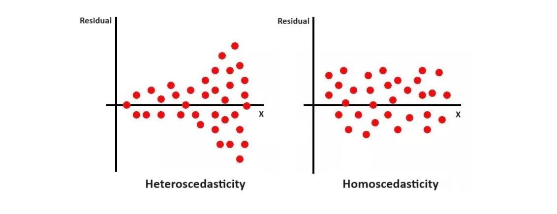
The above is a residual plot of OLS residuals \(\hat\eps_i\) against some explanatory variable \(X\). Notice how for homoscedasticity, the variance of the error terms (how spread out they are up-down wise) is constant for any value of \(X\).
For heteroscedasticity, we can clearly see that the residual variance is smaller for some \(X\) values, and larger for other \(X\) values. If you see a pattern in your residual plot, it is likely heteroscedasticity.
The second way spherical errors can be violated is with autocorrelation, where both of the assumptions of spherical errors are violated.
What is the impact of violating spherical errors?
- OLS estimates remain unbiased. This is because our OLS unbiasedness proof (theorem 4.2) does not depend on the spherical errors assumption.
- Our derived OLS variance is incorrect. This is because our variance formula (theorem 4.3) depends on the spherical errors assumption.
- OLS is no longer the best linear unbiased estimator - the linear unbiased estimator with the lowest variance. This is because the Gauss-Markov Theorem (theorem 4.5) depends on the spherical errors assumption. Thus, there are other linear unbiased estimators with lower variance.
Since OLS remains unbiased, we can still use OLS as an estimator. We just have to correct our OLS variance calculations to account for the fact that spherical errors is not met. There are three different variance formulas used for different forms of non-spherical errors.
Theorem 4.6 (Heteroscedasticity Variance of OLS) The variance of the OLS estimator under heteroscedasticity is given by
\[ \V(\hat{\b\beta}|\b X) = (\b{X^\top X})^{-1}\b X^\top \begin{pmatrix} \sigma^2_1 & 0 & 0 & \dots \\ 0 & \sigma^2_2 & 0 & \dots \\ 0 & 0& \sigma^2_3 & \vdots \\ \vdots & \vdots & \dots & \ddots \end{pmatrix} \b X(\b{X^\top X})^{-1} \]
Proof: Let us start where we left off from eq. 4.2 during the proof of OLS properties. This tells us the variance of the OLS estimator is:
\[ \V(\hat{\b\beta}|\b X) = \V(\b\beta + (\b{X^\top X})^{-1} \b{X^\top \eps}) \]
We know that \(\b\beta\) is a vector of fixed true population values. \((\b{X^\top X})^{-1} \b X^\top\) can also be considered a fixed constant matrix because we are conditioning our variance on \(\b X\). Thus, we can use theorem 1.2 to rewrite the above as
\[ \V(\hat{\b\beta}|\b X) = (\b{X^\top X})^{-1}\b X^\top \V(\b\eps| \b X)[(\b{X^\top X})^{-1}\b X^\top]^{-1} \]
With the properties of matrix inverses and transposes, we can determine that \([(\b{X^\top X})^{-1}\b X^\top]^{-1}\) is equivalent to \(\b X(\b{X^\top X})^{-1}\). Thus, plugging this in, we get
\[ \V(\hat{\b\beta}|\b X) = (\b{X^\top X})^{-1}\b X^\top \V(\b\eps| \b X) \b X(\b{X^\top X})^{-1} \]
Now, we can replace \(\V(\b\eps|\b X)\) with the heteroscedasticity variance matrix of errors:
\[ \V(\hat{\b\beta}|\b X) = (\b{X^\top X})^{-1}\b X^\top \begin{pmatrix} \sigma^2_1 & 0 & 0 & \dots \\ 0 & \sigma^2_2 & 0 & \dots \\ 0 & 0& \sigma^2_3 & \vdots \\ \vdots & \vdots & \dots & \ddots \end{pmatrix} \b X(\b{X^\top X})^{-1} \]
And thus, we have proven the OLS variance under heteroscedasticity. When we actually write the formula, we will typically replace the matrix with \(\b\Omega\).
Clustered standard errors are when you have done clustered sampling for your observations. For example, you randomly sample 100 people from 100 different villages.
The errors of observations belonging to the same cluster (say village) might exhibit correlation, while errors of observtations from distinct clusters are assumed to be uncorrelated.
Definition 4.12 (Clustered Sampling Variance of OLS) The variance of the OLS estimator under clustered sampling is given by
\[ \V(\hat{\b\beta}|\b X) = (\b{X^\top X})^{-1}\b X^\top \begin{pmatrix} \b\Sigma_1 & 0 & \dots & 0 \\ 0 & \b\Sigma_2 & & 0 \\ \vdots & 0 & \ddots & 0 \\ 0 & 0& \dots & \b\Sigma_G \end{pmatrix} \b X(\b{X^\top X})^{-1} \]
Where \(\b\Sigma_1, \dots \b\Sigma_G\) are intracluster covariance-variance error matrices, that exhibit autocorrelation within each cluster, but the different clusters are not autocorrelated.
Proof: Let us start off by taking the same steps as the heteroscedasticity proof, until we got to this point:
\[ \V(\hat{\b\beta}|\b X) = (\b{X^\top X})^{-1}\b X^\top \V(\b\eps| \b X) \b X(\b{X^\top X})^{-1} \]
Now, we can replace \(\V(\b\eps|\b X)\) with the clustered sampling variance matrix of errors:
\[ \V(\hat{\b\beta}|\b X) = (\b{X^\top X})^{-1}\b X^\top \begin{pmatrix} \b\Sigma_1 & 0 & \dots & 0 \\ 0 & \b\Sigma_2 & & 0 \\ \vdots & 0 & \ddots & 0 \\ 0 & 0& \dots & \b\Sigma_G \end{pmatrix} \b X(\b{X^\top X})^{-1} \]
And thus, we have proven the OLS variance under heteroscedasticity. When we actually write the formula, we will typically replace the matrix with \(\b\Omega\).
This type of standard errors is quite complicated, so we usually trust the computer to compute it for us.
Definition 4.13 (HAC Variance of OLS) Heteroscedasticity and Autocorrelation (HAC) variance is given by:
\[ \V(\hat{\b\beta}|\b X) = (\b{X^\top X})^{-1}\b X^\top \b\Omega \b X(\b{X^\top X})^{-1} \]
Where \(\b\Omega\) is the variance-covariance matrix of the error term \(\eps_t\).
Obviously, we probably do not know the form of \(\b\Omega\) ins our population. We can estimate \(\b X^\top \b\Omega \b X\) with the Newey-West Estimator:
\[ \b X^\top \b\Omega \b X = \frac{1}{n}\sum\limits_{t=1}^n \eps_t^2 \b x_t \b x_t^\top + \frac{1}{n}\sum\limits_{\ell = 1}^L \sum\limits_{t = \ell + 1}^n w_\ell\eps_t\eps_{t-\ell}(\b x_t \b x_{t-\ell}^\top + \b x_{t-\ell} \b x_t^\top) \]
Where \(w_\ell\) is given by:
\[ w_\ell = 1 - \frac{\ell}{L + 1} \]
Where \(L\) specifies the maximum lag considered for the control of autocorrelation (so how many previous residuals from previous time periods are correlated with \(\eps_t\)). A common choice for \(L\) is \(n^{1/4}\).
We will not prove this, as it is a very complicated estimator.
Generalised Least Squares
We mentioned that if spherical errors (definition 4.6) is violated, OLS is no longer the linear unbiased estimator with the least variance. Instead, another estimator, the Generalised Least Squares estimator, is the best linear unbiased estimator.
In the generalised least squares estimator, we assume that the variance-covariance is
\[ \V(\b\eps | \b X) = \E(\b{\eps\eps^\top}) = \sigma^2 \b\Omega \tag{4.4}\]
Where \(\sigma^2\) is an unknown scalar constant, but \(\b\Omega\) is a known matrix that is equivalent to the population variance-covariance matrix of errors. The variance is equivalent to \(\E(\b{\eps\eps^\top})\) because we assume by strict exogeneity (definition 4.4) that \(\E(\b\eps) = 0\).
Let us define a matrix \(\b\Omega^{-1/2}\), which will be the inverse of the square root of \(\b\Omega\). This means that the following should be true:
\[ \b\Omega^{-1/2} \ \b\Omega \ {\b\Omega^{-1/2}}^\top = \b I \tag{4.5}\]
We multipy \(\b\Omega^{-1/2}\) to all terms of model \(\b y = \b{X\beta} + \b\eps\) to get a transformed model
\[ \underbrace{\b\Omega^{-1/2}}_{\b y^*} \b y = \underbrace{\b\Omega^{-1/2} \b X}_{\b X^*} \b \beta + \underbrace{\b\Omega^{-1/2} \b \eps}_{\b \eps^*} \tag{4.6}\]
This transformed model meets spherical errors, which we can prove by plugging in the definition of \(\b\eps^*\) from above, and the definition of \(\E(\b{\eps\eps^\top})\) from eq. 4.4:
\[ \begin{align} \V (\b\eps^* | \b X) & = \E(\b\eps^* \b\eps^{*\top}) \\ & = \E(\b\Omega^{-1/2} \b \eps \b\eps^\top {\b\Omega^{-1/2}}^\top) \\ & = \b\Omega^{-1/2} \E(\b{\eps \eps^\top}) \b\Omega^{-1/2} \\ & = \b\Omega^{-1/2} \sigma^2 \b\Omega \b\Omega^{-1/2} \end{align} \]
And by moving scalar \(\sigma^2\) to the front, and using the property from eq. 4.5, we get:
\[ \V (\b\eps^* | \b X) = \sigma^2 \underbrace{\b\Omega^{-1/2} \b\Omega \b\Omega^{-1/2}}_{\b I} = \sigma^2 \b I \]
Thus proving this transformed model meets the spherical errors assumption (definition 4.6). Thus, we can use OLS on this transformed model, and it will be the best linear unbiased estimator. Our OLS estimator (definition 4.8) of the transformed model will be:
\[ \hat{\b\beta} = (\b X^{*\top} \b X^*)^{-1} \b X^{*\top} \b y^* \]
And if we plug in our definitions of \(\b y^*\), and \(\b X^*\) from eq. 4.6, we can get
\[ \hat{\b\beta} = \left[(\b\Omega^{-1/2} \b X)^\top (\b\Omega^{-1/2} \b X) \right]^{-1} (\b\Omega^{-1/2} \b X) (\b\Omega^{-1/2} \b y) \]
And using the properties of matrix transposes, and that \(\b\Omega^{-1/2} \b\Omega^{-1/2} = \b\Omega^{-1}\), we can get
\[ \begin{align} \hat{\b\beta} & = [\b X^\top \b\Omega^{-1/2} \b\Omega^{-1/2} \b X]^{-1} \b X^\top \b\Omega^{-1/2} \b\Omega^{-1/2} \b y \\ & = (\b X^\top \b\Omega^{-1} \b X)^{-1} \b X^\top \b\Omega^{-1} \b y \end{align} \]
Definition 4.14 (Generalised Least Squares Estimator) The GLS estimator is
\[ \hat{\b\beta} = (\b X^\top \b\Omega^{-1} \b X)^{-1} \b X^\top \b\Omega^{-1} \b y \]
Where \(\b\Omega\) is the population variance-covariance matrix of errors. The variance is
\[ \V\hat{\b\beta} = (\b X^\top \b\Omega^{-1} \b X)^{-1} \]
The obvious issue is that we do not generally know the form of \(\b\Omega\). This means the theoretical GLS estimator is often not feasible. Instead, we will use another estimator, called the Feasible Generalised Least Squares (FGLS) estimator.
The only times when GLS is feasible is when we are confident we have a specific form of autocorrelation (such as AR(1), MA(1), which we will cover in the stochastic processes chapter). This is because the covariance-variance matrix is known for these processes, so we can directly use them in GLS.
Feasible Generalised Least Squares
The issue with GLS is that we do not know the form of \(\b\Omega\). Thus, the feasible generalised least squares estimator estimates \(\hat{\b\Omega}\), before estimating the GLS estimator.
There are a few ways we can go about doings this, including the Cochrane-Orcutt Estimator, the Weighted Least Squares estimator, and the 2-stage GLS estimator:
The Cochrane-Orcutt Estimator is a way to estimate GLS assuming autocorrelation of a specific form (Autoregressive 1). Let us start off with a linear model:
\[ Y_t = \beta_0 + \beta_1 X_{t} + \eps_t \]
Let us say some autocorrelation is present - which means the error term \(\eps_t\) is related to some other error term of another observation. More specifically, let us assume an autoregressive order 1 autocorrelation, which means that \(\eps_t\) is correlated with the error term of the time period before, \(\eps_{t-1}\). We can model this as:
\[ \eps_t = \rho \eps_{t-1} + u_t \]
Where \(\rho\) is the coefficient describing the correlation between \(\eps_t\) and \(\eps_{t-1}\), and \(u_t\) is the error term of this smaller model that is the part of \(\eps_t\) that is not explained by \(\eps_{t-1}\).
Thus, our true linear model is:
\[ Y_t = \beta_0 + \beta_1 X_{t} + \rho \eps_{t-1} + u_t \]
If we could get the \(\rho\eps_{t-1}\) term out of this equation, we will no longer have any autocorrelation, since \(u_t\) is not correlated/explained by past error terms.
Consider the linear model for \(Y_{t-1}\):
\[ Y_{t-1} = \beta_0 + \beta_1 X_{t-1}+ \eps_{t-1} \]
Now, let us multiply both sides (every term) with parameter \(\rho\):
\[ \rho Y_{t-1} = \rho\beta_0 + \rho\beta_1 X_{t-1} + \rho\eps_{t-1} \]
Now, let us subtract our model for \(\rho Y_{t-1}\) from our original \(Y_t\):
\[ \begin{array}{ccccccc} Y_t & = & \beta_0 & + & \beta_1X_t & + & \rho\eps_{t-1} + u_t \\ \rho Y_{t-1} & = & \rho\beta_0 & + & \rho\beta_1X_{t-1} & + & \rho\eps_{t-1} \\ \hline Y_t - \rho Y_{t-1} & = & \beta_0(1-\rho) & + & \beta_1(X_t - \rho X_{t-1}) & + & u_t \end{array} \]
Now we can see we have a new transformed model with only error term \(u_t\) which is not autocorrelated with \(t-1\).
\[ \underbrace{Y_t - \rho Y_{t-1}}_{Y_t^*} = \underbrace{\beta_0(1-\rho)}_{\beta_0^*} + \beta_1 \underbrace{(X_t - \rho X_{t-1})}_{X_t^*} + \underbrace{u_t}_{\eps_t^*} \]
Which we can rewrite more simply as:
\[ Y_t^* = \beta_0^* + \beta_1 X_t^* + \eps_t^* \]
Since this model no longer has autocorrelation and now meets spherical errors, we can use the OLS estimator on this transformed model, and this will be the best linear unbiased estimator.
The weighted least squares (WLS) estimator is a FGLS when we have only conditional heteroscedasticity, and we believe that conditional heteroscedasticity to be in a specific form:
\[ \V(\eps_t|\b X) = \sigma^2 \ \Omega(X_t) \tag{4.7}\]
Where \(\sigma^2\) is some constant (can be 1) and \(\Omega(X_t)\) is some function of \(X_t\) that explained the difference in error variance between individuals.
Now, consider the variance of this (modified) error term that is the original error \(\eps_t\) divided by the square root \(\Omega(X_t)\), which is a function of \(X_t\):
\[ \V \left( \frac{1}{\sqrt{\Omega(X_t)}}\eps_t \biggr| X_t \right) \]
Using theorem 1.2, we know \(\V(cu) = c^2 \V(u)\) if \(c\) is a constant and \(u\) is a random variable. This function also applies to a function \(a(x)\) where \(\V(a(x) u) = a(x)^2 \V(u)\). Using this, we can determine the variance of the modified error term is equal to
\[ \V \left( \frac{1}{\sqrt{\Omega(X_t)}}\eps_t \biggr| X_t \right) = \left(\frac{1}{\sqrt{\Omega(X_t)}}\right)^2 \V(\eps_t | X_t) \]
And from eq. 4.7, we can plug in \(\V(\eps_t|X_t) = \sigma^2 \ \Omega(X_t)\) to get
\[ \V \left( \frac{1}{\sqrt{\Omega(X_t)}}\eps_t \biggr| X_t \right) = \frac{1}{\Omega(X_t)}\sigma^2 \ \Omega(X_t) = \sigma^2 \]
What does this tell us? Well it tells us the modified error term \(\frac{1}{\sqrt{\Omega(X_i)}} \eps_t\) has a variance of constant \(\sigma^2\) for all units \(i\), which does not dependent on \(X_i\). What does this mean? Well, our modified error term is now meeting homoscedasticity (definition 4.6)!
However, we obviously cannot just divide the error term by \(1/\sqrt{\Omega(X_t)}\) - that changes our linear model. What we can though do is divide every term of our linear model:
\[ \frac{Y_t}{\sqrt{\Omega(X_t)}} = \beta_0\left(\frac{1}{\sqrt{\Omega(X_t)}}\right) + \beta_1 \left(\frac{X_{t1}}{\sqrt{\Omega(X_t)}}\right) + \dots + \frac{\eps_t}{\sqrt{\Omega(X_t)}} \]
And since we divide both side by \(1/\sqrt{\Omega(X_t)}\), and our model is conditional on individual \(t\) (see all the subscripts), that means this model is still “equivalent” to our original linear model.
Thus, the idea of weighted least squares is to “transform” our heteroscedastic linear model into one that meets homoscedasitcity. We can then just use OLS on our new homoscedastic regression, and since homoscedsaticity is met, Gauss-Markov (theorem 4.5) is met, and our estimator is once again the best linear unbiased estimator.
The previous two methods assumed we know some information about the variance-covariance errors matrix (is there only autocorrelation, or only heteroscedasticity, etc.).
If we do not konw anything, we can still do feasible GLS with a 2-stage process.
We typically produce a estimate \(\hat{\b\Omega}\) by first running an OLS regression, in which we will obtain the residuals \(\hat\eps_i\). These can be used to estimate the structure of \(\b\Omega\), producing \(\hat{\b\Omega}\). Then, using this estimate \(\hat{\b\Omega}\), we can run feasible GLS, and obtain an estimator with less error.
However, this specific form has many drawbacks. When we estimate \(\hat{\b\Omega}\) with OLS (or any other method), we of course have some imprecision in our estimates. Econometricians have shown that the 2-stage feasible GLS estimator often is far worse than the hypothetical perfect GLS. Very often, feasible GLS will actually result in larger variances of estimates.
There is also some risk with 2-stage feasible GLS. Often, heteroscedasticity and autocorrelation occur in our estimated OLS models not because the population actually has heteroscedasticity or autocorrelation, but rather, our original linear model is missing some explanatory variables which causes other violations in our classical linear model, such as exogeneity violations. This mispecified nature will not only make FGLS even more imprecise, but also has the potential to bias FGLS estimates.
Thus, 2-stage FGLS is not super popular in most applied statistician’s toolkit, and the default tends to be sticking to OLS with either robust standard errors or Heteroscedasticity-and-autocorrelation (HAC) robust standard errors.
Instrumental Variables Estimator
One of the assumptions in the classical model is exogeneity (definition 4.4). This assumption is critical in the proofs of OLS unbiasedness and asymptotic consistency. This implies that when exogeneity is violated, our estimates of \(\hat\beta\) become unrealiable.
The instrumental variables estimator is a solution to this issue. The idea is to find a third variable (or more) \(Z\), that does meet this condition of exogeneity:
\[ \E(\b{Z^\top \eps}) = 0 \tag{4.8}\]
and we will have no exogeneity if \(Z\) is not correlated with the error term. We then use these instruments \(Z\) to predict \(X\), which will get us the parts of \(X\) that are explained by \(Z\) (and thus, uncorrelated with the error term). Then, we can use that exogenous part of \(X\) to estimate the relationship with \(Y\). However, this hinges on \(Z\) meeting that moments condition.
Definition 4.15 (Assumptions of Instruments) For instrument(s) \(Z\) to meet the moment condition \(\E(\b{Z^\top \eps}) = 0\), the following facts must be true:
- \(Z\) must be exogenous/ignorable, i.e. \(Cov(Z, \eps) = 0\).
- \(Z\) must be relevant, i.e. \(Cov(Z, X) ≠ 0\).
- \(Z\) must meet the exclusions restriction (which is implied by exogenous). This means that \(Z\) cannot have an independent effect on \(Y\), outside of its impact on \(Y\) through \(X\).
Let us derive the IV estimator (and an alternative IV estimator called 2SLS), and explore the asymptotic properties of this estimator.
So we know what an instrument \(Z\) is, and the requirements for \(Z\) to be a valid instrument. But how does \(Z\) help us estimate the effect between \(X\) and \(Y\)?
Our moment condition and sample equivalent for instrumental variables is:
\[ \E(\b{Z^\top \eps}) \approx \b Z^\top \b\eps = 0 \]
Now, we know that \(\b\eps = \b y - \hat{\b y}\) and \(\hat{\b y} = \b{X\hat\beta}\), so let us plug that in:
\[ \begin{align} \b Z^\top (\b y - \hat{\b y}) & = 0 \\ \b Z^\top (\b y - \b{X \hat\beta}) & = 0 \\ \b{Z^\top y} - \b{Z^\top X \hat\beta} & = 0 \end{align} \]
And now, solving for \(\hat{\b\beta}\) with matrix inversion, we get:
\[ \begin{align} - \b{Z^\top X \hat\beta} & = - \b{Z^\top y} \\ \b{Z^\top X \hat\beta} & = \b{Z^\top y} \\ \hat{\b\beta} & = (\b{Z^\top X})^{-1} \b{Z^\top y} \end{align} \]
Definition 4.16 (Instrumental Variables Estimator) The IV estimator produces the estimates:
\[ \hat{\b\beta}^* = (\b{Z^\top X})^{-1} \b{Z^\top y} \]
Note that the IV estimator is biased in small sample sizes, and only asymptotically consistent (proof provided in the third tab). Thus, we should be careful when using IV in small sample sizes.
It can also be shown that the asymptotic variance of the instrumental variables estimator, under the assumption of spherical errors is
\[ \V \hat{\b\beta}^* = \sigma^2(\b{Z^\top X})^{-1} \b{Z^\top Z} (\b{X^\top Z})^{-1} \]
Although the proof of this is beyond the scope of this chapter. There is also a more complex derivation for robust standard errors with instrumental variables estimation.
While sometimes we do compute the instrumental variables estimator as shown in definition 4.16, often, we use another estimator, the two-stage-least-squares (2SLS) estimator.
The 2SLS estimator is based on the intuitive interpretation of instrumental variables: that we use only the part of \(X\) explained by \(Z\) (which should be endogenous), and estimate that part of \(X\)’s relationship with \(Y\).
The two stage least squares estimator follows this exact procedure. In the first stage, we find the part of \(X\) that is explained by \(Z\), which we call \(\hat X_t\):
\[ \hat X_t = \hat\beta_0 + \hat\beta_1 Z_t \]
We do this by running a linear OLS model with \(X_t\) as the outcome variable, and \(Z_t\) as the explanatory variable. Our predicted \(\hat X_t\) will be the part of \(X\) explained by instrument \(Z\).
Then, for the second stange, we take this \(\hat X_t\), and use it in a model with \(Y\) as follows:
\[ Y_t = \delta_0 + \delta_1 \hat X_t + \eps_t \]
How is 2SLS in these two stages equal to instrumental variables estimator we derived in definition 4.16? Our estimates (in matrix form) for the second stage would be:
\[ \hat{\b\beta}_{2SLS} = (\hat{\b X}^\top \hat{\b X})^{-1} \hat{\b X}^\top \b y \tag{4.9}\]
Where \(\hat{\b X}\) is given as the fitted values of the first stage:
\[ \hat{\b X} = \b Z \hat{\b \delta} = \b Z (\b{Z^\top Z})^{-1}\b{Z^\top X} \]
We can plug \(\hat{\b X}\) into eq. 4.9 to get:
\[ \hat{\b\beta}_{2SLS} = [(\b Z (\b{Z^\top Z})^{-1}\b{Z^\top X})^\top (\b Z (\b{Z^\top Z})^{-1}\b{Z^\top X})]^{-1}(\b Z (\b{Z^\top Z})^{-1}\b{Z^\top X})^\top \b y \]
Using the properties of matrix transposes, we get:
\[ \begin{align} \hat{\b\beta}_{2SLS} & = [(\b X^\top \b Z (\b{Z^\top Z})^{-1} \b Z^\top) (\b Z (\b{Z^\top Z})^{-1}\b{Z^\top X})]^{-1}(\b X^\top \b Z (\b{Z^\top Z})^{-1} \b Z^\top)\b y \\ & = [\b X^\top \b Z \underbrace{(\b{Z^\top Z})^{-1} \b Z^\top \b Z}_{\text{inverses cancel}} (\b{Z^\top Z})^{-1}\b{Z^\top X}]^{-1}\b X^\top \b Z (\b{Z^\top Z})^{-1} \b Z^\top\b y \\ & = (\underbrace{\b X^\top \b Z (\b{Z^\top Z})^{-1}}_{\text{cancel}}\b{Z^\top X})^{-1}\underbrace{\b X^\top \b Z (\b{Z^\top Z})^{-1}}_{\text{cancel}} \b Z^\top\b y \\ & = \underbrace{(\b{Z^\top X})^{-1} \b{Z^\top y}}_{\text{equal to IV}} \end{align} \]
And the second to last step is possible because one of the highlighted “cancel” parts is within an inverse and the other isn’t, so they cancel. Thus, we have shown 2SLS is equivalent to the instrumental variables estimator.
Despite being biased, the instrumental variables estimator is an asymptotically consistent estimator of \(\b\beta\) even with exogeneity between \(X\) and \(\eps\) violated (as long as \(Z\) is exogenous).
Theorem 4.7 (IV Consistency) The IV estimator is asymptotically consistent, meaning
\[ \mathrm{plim}\hat{\b\beta}^* = \b\beta \]
Proof: Let us first re-arrange the IV estimator by plugging in the original model \(\b y = \b{X\beta} + \b\eps\), and simplify:
\[ \begin{align} \hat{\b\beta}^* & = (\b{Z^\top X})^{-1} \b{Z^\top y} \\ & = (\b{Z^\top X})^{-1} \b{Z^\top}(\b{X\beta} + \b \eps) \\ & = \underbrace{(\b{Z^\top X})^{-1} \b{Z^\top X}}_{\text{inverses cancel}}\b\beta + (\b{Z^\top X})^{-1} \b{Z^\top\eps} \\ & = \b\beta + (\b{Z^\top X})^{-1} \b{Z^\top\eps} \end{align} \]
We can rewrite our matrices in the form of vectors, scalars, and summation:
\[ \begin{align} \hat{\b\beta}^* & = \b\beta + (\b{Z^\top X})^{-1} \b{Z^\top\eps} \\ & = \b\beta + \left(\sum\limits_{t=1}^n \b z_t \b x_t^\top \right)^{-1} \left(\sum\limits_{t=1}^n \b z_t \eps_t \right) \end{align} \]
Now, let us do a little algebra trick as follows:
\[ \hat{\b\beta}^* = \b\beta + \left(\frac{1}{n}\sum\limits_{t=1}^n \b z_t \b x_t^\top \right)^{-1} \left(\frac{1}{n}\sum\limits_{t=1}^n \b z_t \eps_t \right) \]
The reason we can do this is because the first \(\frac{1}{n}\) is inversed as \(\frac{1}{n}^{-1}\), so this cancels out the second one, maintaining the equality of our equation.
Now, we want to prove \(\mathrm{plim}\hat{\b\beta}^* = \b\beta\), so let us take the probability limit of both sides:
\[ \mathrm{plim}\hat{\b\beta}^* = \mathrm{plim}\b\beta + \left(\mathrm{plim}\frac{1}{n}\sum\limits_{t=1}^n \b z_t \b x_t^\top \right)^{-1} \left(\mathrm{plim}\frac{1}{n}\sum\limits_{t=1}^n \b z_t \eps_t \right) \]
We know the probability limit of a constant is itself. Look at the other two terms on the right: they take the form of sample averages \(\frac{1}{n}\sum\). Using the law of large numbers (theorem 2.1), we can simplify to:
\[ \mathrm{plim}\hat{\b\beta}^* = \b\beta + (\E(\b z_t \b x_t^\top))^{-1} \underbrace{\E(\b z_t \eps_t)}_{= \ 0} = \b\beta \]
And we know \(\E(\b z_t \eps_t) = 0\) because this is the same condition as the moment condition \(\E(\b{Z^\top \eps}) = 0\), just written in terms of individual observations. Thus, the Instrumental variables estimator is asymptotically consistent.
Statistical Inference
Standard errors are by definition, the square root of the variance of the estimator, which we derived for both OLS under spherical errors, and OLS under non-spherical errors.
There is an issue though: \(\sigma^2\) is the population variance of error term \(\eps_i\), and appears in the OLS variance under spherical errors. But we don’t know this population value. Thus, we will need an estimator \(s^2\) that will estimate \(\sigma^2\):
\[ s^2 = \frac{\b{\hat\eps^\top \hat\eps}}{n - p-1} = \frac{\sum_{t=1}^n \hat\eps_t^2}{n-p-1} \]
Where \(\hat{\b\eps}\) are equal to \(\b y - \hat{\b y}\), and can be calculated with residual maker \(\b M\) as shown in eq. 4.1. \(n\) is the size of our sample, and \(p\) is the number of explanatory variables we have. We will not prove it here, but this is an unbiased estimator of \(\sigma^2\)
For OLS variance in conditional heteroscedasticity (robust), we have the unknown population term \(\sigma^2_i\), which we estimate with \(s^2_i\):
\[ \sigma^2_i \approx s^2_i = \hat\eps_i^2 \]
However, our estimate \(s^2\) and \(s_i^2\) has an implication - every estimator has variance and uncertainty.
Under the central limit theorem (theorem 2.2), our standardised sampling distribution of \(\hat\beta_j\) should be normally distributed. However, because we are estimating \(\sigma^2\) with \(s^2\), this uncertainty in estimates \(s^2\) means we cannot use the normal distribution as given by the central limit theorem. Instead, we use a t-distribution to account for the uncertainty.
Once we have our correct standard errors, we can conduct hypothesis testing. There are two main hypothesis tests: the t-test for single parameters, and the f-test for multiple parameters or comparing models:
The t-test is a way to test single parameters in our linear model. Typically, our hypothesis are the following:
- \(H_0: \beta_j = 0\), which states that there is no relationship between \(X_j\) and \(Y\).
- \(H_1: \beta_j ≠ 0\), which states that there is a relationship between \(X_j\) and \(Y\).
Definition 4.17 (T-Test) In our t-test, our test statistic is the t-statistic.
\[ t = \frac{\hat\beta_j - \text{null value}}{se(\hat\beta_j)} \]
And we will conduct a hypothesis test using the \(t\)-distribution with degrees of freedom of \(n-p-1\).
We then calculate a p-value. The procedure of conducting a hypothesis test was outlined in the last chapter. If our p-value is statistically significant, we can conclude there is a significant relationship between \(X_j\) and \(Y\).
We can also do a statistical inference test with multiple coefficients at a time with the F-test. The F-test compares two different models, a null model with less parameters, and a alternate model with all the parameters in the null and some more parameters:
\(M_0 : Y_t = \beta_0 + \sum\limits_{j=1}^g \beta_j X_{tj} + \eps_t\) (the smaller null model with \(g\) parameters).
\(M_a : Y_t = \beta_0 + \sum\limits_{j=1}^g \beta_j X_{tj} + \sum\limits_{j=g+1}^p \beta_j X_{tj} \eps_t\) (the bigger model with the original \(g\) parameters in the null + additional parameters up to \(p\)).
Recall \(R^2\) (definition 4.11), which is a measure of fit for our models. F-tests compare the \(R^2\) of the alternate model to the null model.
Definition 4.18 (F-test) F-tests are used to test a smaller model \(M_0\) and larger model \(M_a\) model. The F-test statistic is given by
\[ F = \frac{(SSR_0 - SSR_a) / (p_a - p_0)}{SSR_a /(n-p_A - 1)} \]
Where \(SSR\) represents the sum of squared residuals, \(p\) represents the number of parameters in each model, and \(n\) is the sample size (should be the same between both \(M_0\) and \(M_a\)).
We then consult a F-distribution with \(p_1 - p_0\) and \(n - p_a - 1\) degrees of freedom.
We then calculate a p-value. The procedure of conducting a hypothesis test was outlined in the last chapter.
If our result is statistically significant, then the alternative model \(M_a\) is a statistically significantly better model than \(M_0\), and the extra parameters in \(M_a\) are jointly significant.